This post is about our recently accepted BMVC2017 paper (pdf, slides, poster) as oral presentation (and Best industrial paper award), I will try to summarize the ideas of our work.

In a few lines:

We propose a novel Stixel depth model (Slanted Stixels) that represents non-float roads better than previous methods but it is also slower. To keep it real-time, we also introduce an approximation that uses an over-segmentation of “Stixel Cuts” to speed up the algorithm maintaining similar performance, this trick can also be applied to previous dynamic programming Stixel methods.

Example results on real-world San Francisco data:

More details:

Motivation

The Stixel World has been successfully used for representing traffic scenes. It defines a compact medium-level representation of dense 3D disparity data obtained from stereo vision using rectangles (Stixels) as elements. These are classified either as ground-like planes, upright objects or sky, which are the geometric primitives found in man-made environments. This converts millions of disparity pixels to hundreds or thousands of Stixels. At the same time, most task-relevant scene structures, such as free space and obstacles, are adequately represented.

Our work yields an improved Stixel representation that accounts for non-flat roads, outperforming the original Stixel model in this context while keeping the same accuracy on flat road scenes.

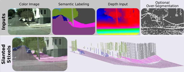The proposed approach: pixel-wise semantic and depth information serve as input to our Slanted Stixels, a compact semantic 3D scene representation that accurately handles arbitrary scenarios as e.g. San Francisco. The optional over-segmentation in the top-right yields significant speed gains nearly retaining the depth and semantic accuracy.

State of the art

Stixels were originally devised to represent the 3D scene as observed by stereoscopic or monocular imagery. Our proposal is based on Semantic Stixels: they use semantic cues in addition to depth to extract a Stixel representation. However, they are limited to flat road scenarios due to constant height assumption. In contrast, our proposal overcomes this drawback by incorporating a novel plane model together with effective priors on the plane parameters.

Some methods model the scene with a single Stixel per column: they can be faster but provide an incomplete world model, e.g. they cannot represent a pedestrian and a building in the same column. There are also FPGA and GPU implementations running Stixels at real-time. In contrast, we propose a novel algorithmic approximation that is hardware agnostic. Accordingly, it could also benefit of the aforementioned approaches.

Brief Stixel model description

The Stixel world is a segmentation of image columns into stick-like super-pixels with class labels and a 3D planar depth model. This joint segmentation and labeling problem is carried out via optimization of the column-wise posterior distribution \(P(S: | M:)\) defined over a Stixel segmentation \(S:\) given all measurements \(M:\) from that particular image column. In the following, we drop the column indexes for ease of notation.

A Stixel column segmentation consists of an arbitrary number \(N\) of Stixels \(S_i\), each representing four random variables: the Stixel extent via bottom \(V_i^b\) and top \(V_i^t\) row, as well as it’s class \(C_i\) and depth model \(D_i\). Thereby, the number of Stixels itself is a random variable that is optimized jointly during inference.

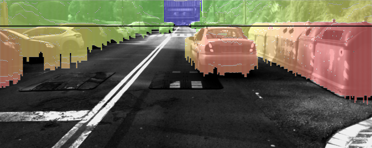Example of Stixel World estimation. Sky stixels are represented on blue, object stixels are represented on green-to-red (read= close, green= far), and ground stixels are transparent.

To this end, the posterior probability is defined by means of the unnormalized prior and likelihood distributions \(P(S: \| M:) = \frac{1}{Z} P(M \| S)P(S)\) transformed to log-likelihoods via \(P(S = s \| M = m) = - log(e^{-E(s,m)})\).

The likelihood term \(E_{data}(\cdot)\) thereby rates how well the measurements \(m_v\) at pixel \(v\) fit to the overlapping Stixel \(s_i\)

This pixel-wise energy is further split in a semantic and a depth term

The semantic energy favors semantic classes of the Stixel that fit to the observed pixel-level semantic input. The parameter \(w_l\) controls the influence of the semantic data term. The depth term is defined by means of a probabilistic and generative sensor model \(P_v(\cdot)\) that considers the accordance of the depth measurement \(d_v\) at row \(v\) to the Stixel \(s_i\)

It is comprised of a constant outlier probability \(p_{out}\) and a Gaussian sensor noise model for valid measurements with confidence \(c_v\)

that is centered at the expected disparity \(\mu(s_i,v)\) given the depth model of the Stixel. \(Z_{U}\) and \(Z_G(s_i)\) normalize the distributions.

The prior captures knowledge about the segmentation: the Stixel segmentation has to be consistent, i.e. each pixel is assigned to exactly one Stixel. A model complexity term favors solutions composed of fewer Stixels by invoking costs for each Stixel in the column segmentation S. Furthermore, prior assumptions as “objects are likely to stand on the ground” and “sky is unlikely below the road surface” are taken into account. The interested reader is referred to the original Stixel paper for more details. The Markov property is used so that the prior reduces to pair-wise relations between subsequent Stixels. This energy function is optimzed by Dynamic Programming.

Our contribution

1. New depth model

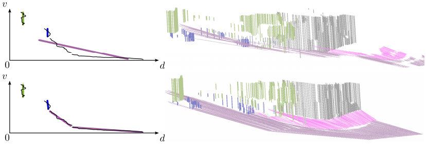Comparison of original (top) and our slanted (bottom) Stixels: due to the fixed slant in the original formulation the road surface is not well represented as illustrated on the left. The novel model is capable to reconstruct the whole scene accurately.

This paper introduces a new plane depth model that overcomes the previous rather restrictive constant depth and constant height assumptions for object respectively ground Stixels. To this end, we formulate the depth model \(\mu(s_i, v)\) using two random variables defining a plane in the disparity space that evaluates to the disparity in row \(v\) via

Note that we assume narrow Stixels and thus can neglect one plane parameter, i.e. the roll.

We also propose a new additional prior term that uses the specific properties of the three geometric classes. We expect the two random variables A,B representing the plane parameters of a Stixel to be Gaussian distributed, i.e.

This prior favors planes in accordance to the expected 3D layout corresponding to the geometric class. i.e. object Stixels are expected to have an approximately constant disparity, i.e. \(\mu_{\textit{object}}^{b} = 0\). The expected road slant \(\mu_{\textit{ground}}^{a}\) can be set using prior knowledge or a preceding road surface detection. Note that the novel formulation is a strict generalization of the original method, since they are equivalent, if the slant is fixed, i.e. \(\sigma_{object}^{b} \rightarrow 0, \mu_{object}^{b} = 0\).

We have to optimize jointly for the novel depth model. When optimizing for the plane parameters \(a_i,b_i\) of a certain Stixel \(s_i\), it becomes apparent that all other optimization parameters are independent of the actual choice of the plane parameters. We can thus simplify

Thus, we minimize the global energy function with respect to the plane parameters of all Stixels and all geometric classes independently. We can find an optimal solution of the resulting weighted least squares problem in closed form, however, we still need to compare the Stixel disparities to our new plane depth model. Therefore, the complexity added to the original formulation is another quadratic term in the image height.

2. Stixel Cut Prior

The Stixel inference described so far requires to estimate the costs for each possible Stixel in an image, although many Stixels could be trivially discarded, e.g. in image regions with homogeneous depth and semantic input. We propose a novel prior that can be easily used to significantly reduce the computational burden by exploiting hypothesis generation. To this end, we formulate a new prior, but instead of Stixel bottom and top probabilities we incorporate generic likelihoods for pixels being the cut between two Stixels. We leverage this additional information adding a novel term for a Stixel \(s_i\)

where \(c_{v_i^b}(cut)\) is the confidence for a cut at \(v_i^b\) thus \(c_{v_i^b}(cut) = 0\) implies that there is no cut between two Stixels at row \(v\).

Our method trusts that all the optimal cuts will be included in our over-segmentation, therefore, only those positions are checked as Stixel start and end. This reduces the complexity of the Stixel estimation problem for a single column to \(\mathcal{O}(h' \times h')\), where \(h'\) is the number of over-segmentation cuts computed for this column, \(h\) is image height and \(h' \ll h\).

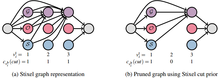Stixel inference illustrated as shortest path problem on a directed acyclic graph: the Stixel segmentation is computed by finding the shortest path from the source (left gray node) to the sink (right gray node). The vertices represent Stixels with colors encoding their geometric class, i.e. ground, object and sky. Only the incoming edges of ground nodes are shown for simplicity. Adapted from this paper

The computational complexity reduction becomes apparent the last figure. The inference problem can be interpreted as finding the shortest path in a directed acyclic graph. Our approach prunes all the vertices associated with the Stixel’s top row not included according to the Stixel cut prior.

New dataset

We introduce a new synthetic dataset inspired by Synthia. This dataset has been generated with the purpose of evaluating our model (it includes non-flat roads), but it contains enough information to be useful in additional related tasks, such as object recognition, semantic and instance segmentation, among others. SYNTHIA-San Francisco (SYNTHIA-SF) consists of photorealistic frames rendered from a virtual city and comes with precise pixel-level depth and semantic annotations for 19 classes. This new dataset contains 2224 images that we use to evaluate both depth and semantic accuracy.

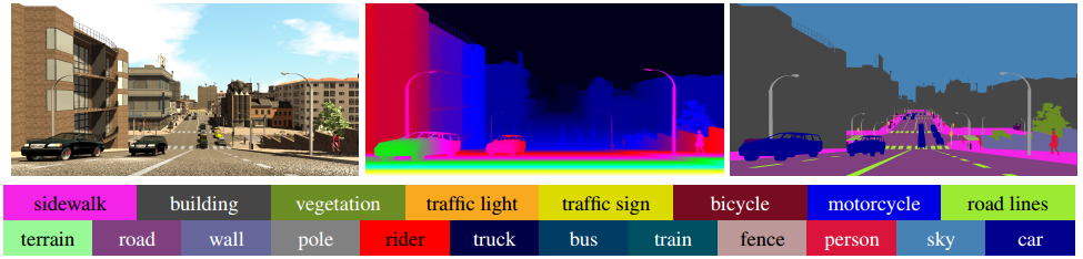The SYNTHIA-SF Dataset. A sample frame (left) with its depth (center) and semantic labels (right)

Results

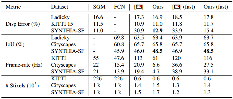Quantitative results of our methods compared to original Stixels [23], raw SGM and FCN. Signifi- cantly best results highlighted in bold.

The first observation is that all variants are compact representations of the surrounding, since the complexity of the Stixel representation is small compared to the high resolution input images, c.f. the last row of the table.

Second, our method achieves comparable or slightly better results on all datasets with flat roads. This indicates that the novel and more flexible model does not harm the accuracy in such scenarios.

The third observation is that the proposed fast variant improves the run-time of both the original Stixel approach by up to 2x and the novel Stixel approach by up to 7x with only a slight drop in depth accuracy. The benefit increases with higher resolution input images. This is due to the mean density of Stixel cuts in our over-segmentation for SYNTHETIC-SF of 13% with standard deviation of 2, which is equivalent to a 8x reduced vertical resolution.

Finally, we observe that our novel model is able to accurately represent non-flat scenarios in contrast to the original Stixel approach yielding a substantially increased depth accuracy by more than 17%. We also improve in terms of semantic accuracy, which we address to the joint semantic and depth inference that benefits of a better depth model.

Acknowledgements

This research has been supported by the MICINN under contract number TIN2014-53234-C2-1-R. By the MEC under contract number TRA2014-57088-C2-1-R and the Generalitat de Catalunya projects 2014-SGR-1506 and 2014-SGR-1562, we also thank CERCA Programme / Generalitat de Catalunya, NVIDIA for the donation of the systems used in this work and SEBAP for the internship funding program. Finally, we thank Francisco Molero, Marc García, and the SYNTHIA team for the dataset generation.